Data is often imperfect
As consultants we know that perfect data is a myth. No matter the organization or website, data is gunky, irregular, and often broken.
Was at Starbucks this morning doing my travel and expenses. Went to the American Express website and downloaded the last 6 months of corporate charges, or about $34K in planes, hotels, rental cars, Fedex prints, and restaurant bills. So far so good.
Oddly, the sums did not match my records. Hmmmm. After a little bit of sorting and filtering, I saw that there were duplicate expenses. Come on Amex, what’s up?
How to eliminate duplicate data in excel?
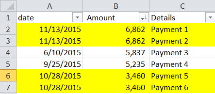
There were about 370+ expenses, of which 1 in 5 were duplicates (same date, same vendor, same amount). Sorted by $ amount and you can see the sporadic duplicates. Oddly, only some were duplicates. Sheesh.

The novice approach would be to eye-ball the duplicates and selectively start deleting. Obviously that is a weak and fallible approach. Trust me. . .this kind of ad-hoc data clean up happens all the time in corporate America. It’s okay when you have 15 rows of data, but what happens with you have 24,000 rows? Need scale, need auditing.
Note: there is a data –> remove duplicate function. Super easy, but you can’t really audit the blackbox functionality, the rows just “disappear”. Therefore, this is a more laborious, but also trackable way to do it.
1. CONCATENATE
Not an excel formula you use often, but super useful; it simply combines two cells into 1 cell. In this example, we are just combining “apple” + “watch” to get “applewatch”. Ta-da. Simple, a bit boring, but trust me, useful.
For my file, I combined column A (date) + column B (amount) to get an unique id; The two YELLOW cells became the ORANGE cell. Copy down, all rows get a unique id.
2. SORT
Then I sorted the file by my new new id to put things in order (column D).
- Data –> Sort (this might look different depending on your MS Office version)
- Or you can do what excel wizards do. . .[ALT] D, F, F.
3. IF statement
This is something analysts use all the time.
- The formula works like this: = if (A relationship B, then C, if not then D)
- One example: if the test score is greater than 75, I am happy, if not I am sad
For my file, I told the excel to see if the cell was the same as the one directly below it. (Remember I SORTED them in order). If ORANGE = YELLOW, then 1, if not 0.
Copy down, this is what your get. . . a series of 1 = yes duplicate, 0 = not duplicate.
4. Copy / Paste as Values
This is a critical step lots of newbies miss (trust me I have made this mistake 100 times). . . copy the newly created formula columns and PASTE AS VALUES. This is how you keep the 1s and the 0s matched up the correct rows.
5. Sort by Duplicates
Since the 1s are duplicates, you can sort again and see there are 79 duplicates. If you eliminate those, then you have clean data.
6. Caveat #1
This method is not infallible because you conceivably could have legitimate expenses which were the same date & amount. Perhaps a “safer” way to go would be to also concatenate the vendor.
7. Caveat #2
When you are cleaning data, I recommend that you:
- Keep 1 tab of your original data, and just copy data over to a new worksheet
- What ever you remove from the old data set, “cut” and paste on a different tab
To newbies. Let me know if you want a copy of the source data to play with.
To excel wizards: I know this was rudimentary. Let me know what other quick tips you have for deleting duplicates in data?
P.S. In the comments, Kevin noted that there is a REMOVE DUPLICATE function in Excel. . under Data –> Data Validation. In the exercise above, you will want to keep the original file to make sure you can audit what the “blackbox” functions are doing.
